The following pictures show the operation of a single-phase LAr TPC. Source*

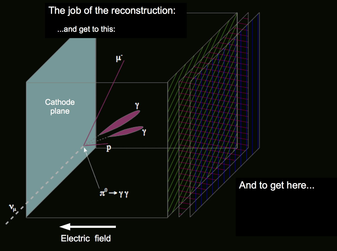
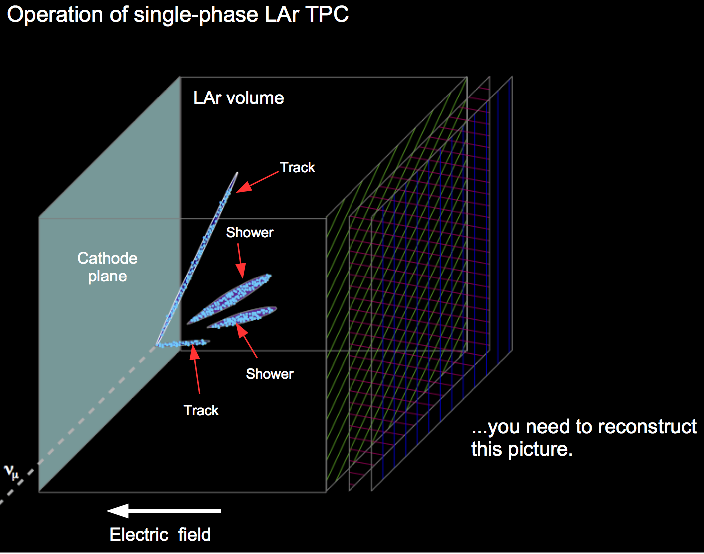
LArTPCs provide bubble chamber quality images in a digital format. Automated reconstruction in liquid argon is not a simple task. Events are complicated topologically with tracks and showers developing side-by-side in the same detector volume. Interactions can start anywhere throughout the volume which makes the start-point of events uncertain. The high density of energy deposits can be very detailed, presenting a challenge for efficient reconstruction. Multiple scattering occurs throughout the volume continuously. Reconstruction starts with the digital information to get to a representation of what occurred when the event happened as shown in the following pictures.

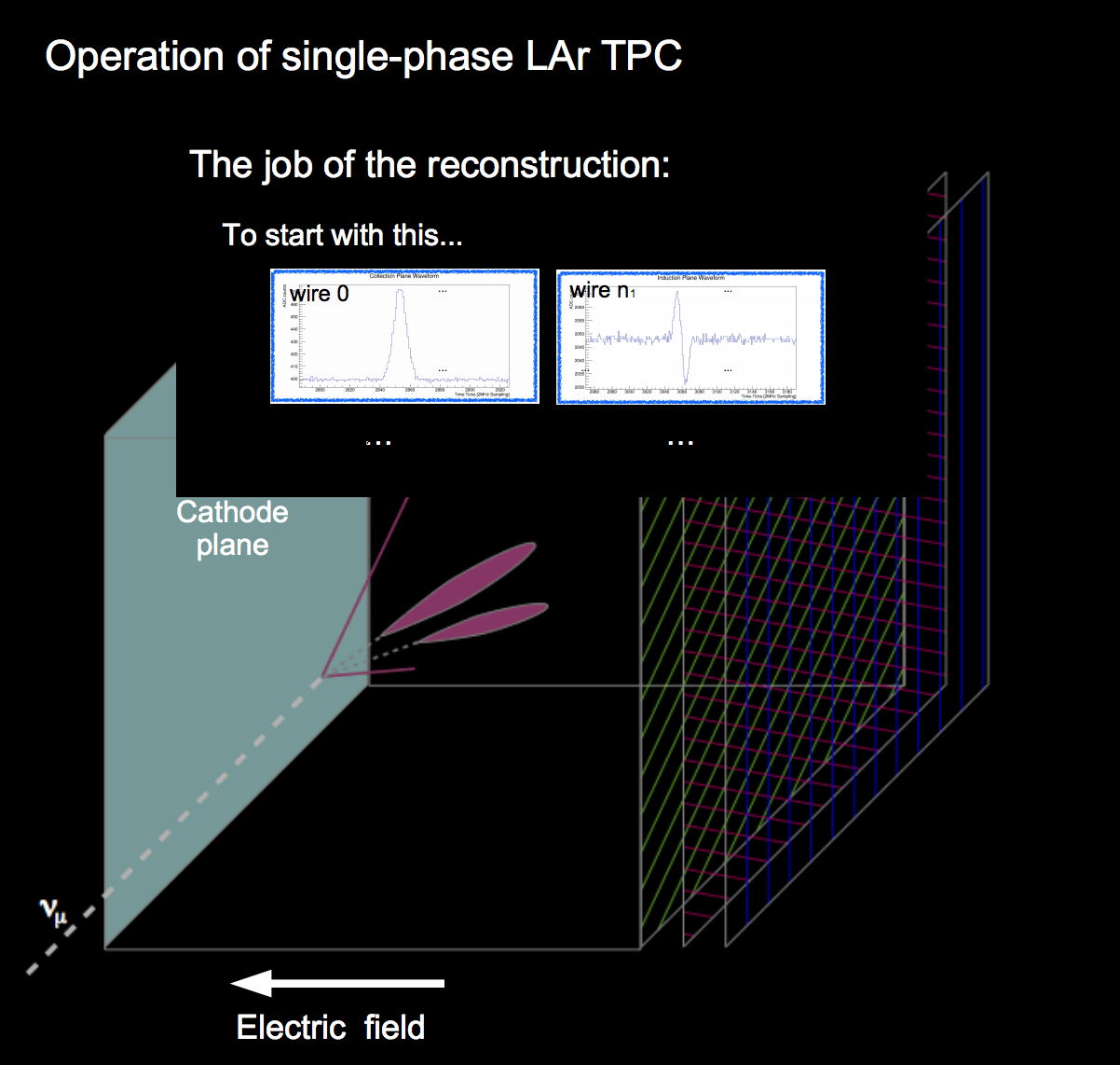
This requires understanding the reconstruction workflow and data structures. As new algorithms are developed, the workflow may change. For now, start with wire data that represents a wave form on a channel.

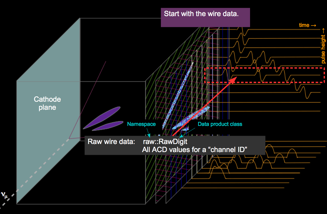
Now need to look for signals associated with particles in the LAr dealing with the problems that induction plane signals are completely different from those on collection wires and RawDigits are not calibrated.

Signal processing

The purpose of signal processing is to prepare raw signals for the second step in reconstruction. Signal processing is applied to the raw waveform. The raw waveform is not just the TPC signal. It also has noise plus the effects of the electronics response function plus a pedestal offset. The pedestal offset is removed by the first step of calibration. Given the impulse response of the front-end electronics and the estimated mean power spectrum for the signal and noise, a measured signal can be deconvoled to get the estimate for the signal which has the optimal value of the signal to noise. It’s not guaranteed to preserve normalization. Note: this isn’t the only type of signal processing that occurs. Extracting optional estimate is optimized for signal-to-noise. It doesn’t preserve the pulse height. Deconvolution is the inverse of the following problem:

This is the only way to optimize for signal-to-noise. After signal processing, the waveform for a single channel is stored in a new data product called recob::Wire.

Hit finding

Hit finding, in general terms, groups together ADC (Analog to Digital Converter) values on each wire that correspond to the ionization associated with a single particle as it traverses the measurement volume for that wire. (Not exactly, but close enough.) In the following picture, all hits are attributed to a single physical entity, (relative) start/end position, some shape parameters.

Hits (recob::Hit) represent the charge deposition by a single particle on that channel. Hit finding is not concerned with finding the actual position of the track in the detector. Found hits are used later in reconstruction to determine the distance at which the track traverses the wire plane, i.e. the actual position of the hit. Particles leave different amounts of energy depending on their speed. The charge in the hit gives an estimate of the energy deposition within the measurement volume of the wire.

The output of hit-finding:    
recob::Hit + Assns<Wire,Hit>, Assns<RawDigit,Hit>

All ADC values on a given wire attributed to a single particle, and the arrival time of ionization relative to a common (arbitrary) t0 Hit-finding is performed by:

• CCHitFinder
• GausHitFinder
• RFFHitFinder
• …

Hits are grouped into clusters that represent the ionization of a single physical entity.

This clustering procedure is (usually) performed in 2D. Clusters are groups of hits that are associated in time and space. Can use Harris transform (image processing technique) to identify end points in 2D views as seeds for clusters. Several clustering techniques are in use. Can identify straight lines using a Hough transform and arbitrary shapes using a density-based algorithm.

The output of 2D clustering is:
recob::Cluster + Assns<Hit,Cluster>

 

At least one 3D clustering algorithm, Cluster3D, produces associated 2D recob::Cluster objects among other things. Cluster finding is across channels, finding the hits that belong to the ionization from a single physical entity. Could be a shower so it may not be a single channel. The clusters may be representing the cascading, not the individual tracks.

Given the 2D clusters, can now combine them into 3D objects, tracks or showers.

The output of tracking:   
 recob::Track + Assns<Cluster,Track> 
    Estimated points + direction + covariance along trajectory
        Tracks can also have associated recob::Vertex objects
        and recob::PFParticle objects (preliminary particle flow hypotheses)

Clusters from multiple views are merged into either tracks or showers. Merging requires knowledge of the timing in each view.

Tracking algorithms:

• Track3DKalman∗
• CCTrackMaker
• CosmicTracker
• …

 

Clusters can also be part of showers. Finding shower-like clusters is sometimes done at the same time as the shower-finding itself. This is usually the start of calorimetric measurements.

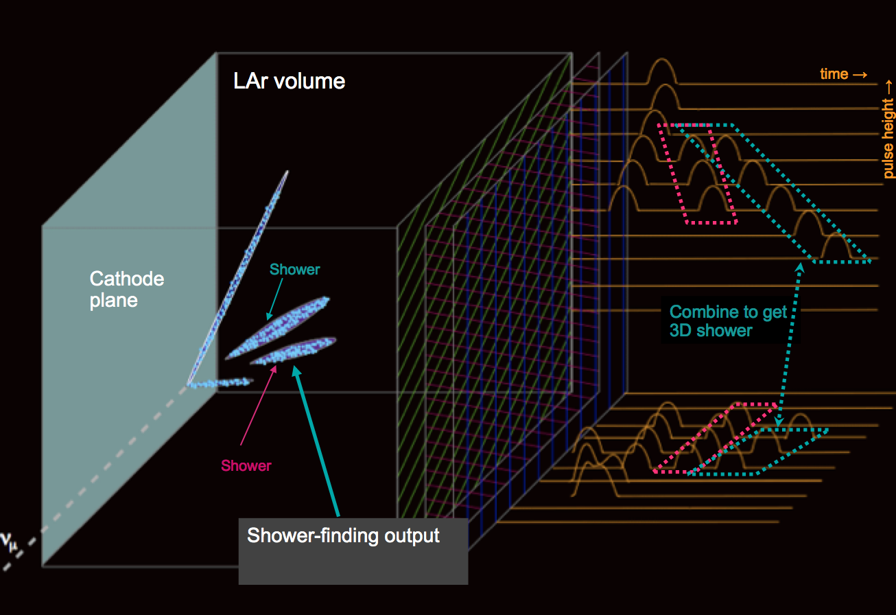
Shower-finding output:    
  recob::Shower + anab::Calorimetry
  Assns<Cluster,Shower> + Assns<Hit,Shower>
  Shower parameters, energy estimates

Shower-finding algorithms:

• ShowerFinder
• ShowerReco
• ShowerReco3D
• …

Scintillation light is used to determine the interaction time in a procedure called flash-finding. Without the interaction t0, the absolute position of energy deposition
cannot be determined. Start with Optical raw data: raw::OpDetWaveform
Optical reconstruction starts with hit-finding (analogous to wire hit-finding), followed by flash-finding, which estimates interaction t0.

Flash-finding output:  
         recob::OpHit + recob::OpFlash
         Pulse heights, arrival times, event t0, flash centroid

Flash-finding algorithms:
OpFlashAlg

There are other steps, these are covered in the Secondary reconstruction.

Analysis-phase reconstruction

Cosmic ray removal is particularly important for surface detectors such as SBN detectors at Fermilab and Test Beam detectors. Cosmic ray removal employs track-finding, clustering, flash-track and flash-cluster matching.
Representative algorithms:

• CosmicTrackTagger,
• BeamFlashTrackMatchTagger
• …

Output:  
anab::CosmicTag

Calorimetric measurements are energy and dE/dx estimates for tracks.
Representative algorithms: * CalorimetryAlg, * TrackCalorimetryAlg

Output:  
anab::Calorimetry

Momentum estimation and particle identification uses range, dE/dx and multiple Coulomb scattering of tracks.
Representative algorithms:

• Chi2PIDAlg,
• PIDAAlg

  Output:  
  anab::ParticleID, Assns<Track, ParticlePID>, or TTree

Other Complications

There are other complications such as space-charge distortions, charge attenuation, hit disambiguation and dual-phase LAr TPCs.

Space-charge distortions

There can be a build-up of slow-moving positive ions in a detector due to ionization from cosmic rays. This leads to a distortion of the
electric field within the detector, and a displacement in the reconstructed position of signal ionization electrons in LArTPC detectors.
Ion drift mobilities are about 106× smaller than that of electrons; Cation drift velocities are ~nm / μs.
High cosmic ray rate for surface detectors introduces significant positive ion load. Need to map and correct for these. A common service in LArSoft exists to access the offsets

Charge attenuation

Electron lifetime can be comparable to maximum drift time. Effective gain will be drift-length dependent. Expect to see significant reduction in SNR with drift distance.

This is based on the material from Introduction to LArSoft – source material.